Usage

Introduction

The code uses MHD simulation results to evolve the particle distribution functions according to the transport equations. The MHD quantities used include magnetic field, velocity field, and maybe plasma density.

Note

The plasma density might be used to calculate the local Alfvén speed.

In general, the modeling procedure includes

Run the MHD simulations and get the MHD fields.
Pre-process the MHD results to provide the input data for the GPAT model.
Calculate the input parameters, including the spatial diffusion coefficient, parameters for evaluating the momentum diffusion coefficient, parameters for evaluating the particle drift, etc.
Modify the configuration for the transport modeling.
Run the simulation.
Analyze and visualize the results.

Below, we will use a 2D magnetic reconnection problem to illustrate the procedure in more detail.

Example: 2D Magnetic Reconnection

Here, we use a 2D reconnection problem solved with Parker’s transport equation as an example. The relevant code and scripts are in examples/reconnection_2d.

Note

More examples will be included in the future.

Run the MHD simulation

Please follow the instructions in athena_reconnection to run a reconnection simulation with two current sheets and periodic boundary conditions. The input file for the Athena++ simulation is code/athinput.reconnection in athena_reconnection. The simulation domain size is [0, 2] $\times$ [0,2]. The grid size is $1024\times1024$. The simulation will last 20 Alfven-crossing time and produce 200 frames of data of the primary variables (reconnection.prim*.athdf) in default.

Pre-process the MHD data

Instead of directly processing the data from different MHD codes (e.g., VTK files by Athena and HDF5 files by Athena++) in the simulations, we will reorganize the MHD simulation outputs using Python scripts first. The example scripts for Athena and Athena++ outputs are in mhd_data. There is a shell script reorganize_data.sh for running the Python scripts with commandline arguments.

./reorganize_data.sh

which will include 2 ghost cells at each boundary according to the boundary conditions (periodic or open).

Note

Due to their stochastic nature, the pseudo particles can cross the local domain boundaries multiple times in a short time, significantly increasing the MPI communication cost. We choose two ghost cells to enable particles to stay in the local domain when they are near the boundaries. The two ghost cells also make calculating the gradients of the fields easier at the boundaries. This could be improved in the future.

The script will generate the MHD fields (in bindary format) and the simulation configuration needed for the transport modelings in bin_data under the MHD run directory.

mhd_data_*: $v_x, v_y, v_z, \rho, B_x, B_y, B_z, B$, which have a size of $1028\times1028$.
rho_*: plasma density ($1028\times1028$)
pre_*: plasma pressure ($1028\times1028$)
mhd_config.dat: the MHD configuration information. See the function save_mhd_config in mhd_data/reorganize_fields.py for the details of the configuration.

Calculate the input parameters

Before transport modeling, we need to calculate the parallel diffusion coefficient $\kappa_\parallel$ using the simulation normalizations (length scale, magnetic field, plasma density, turbulence amplitude and anisotropy). There is a Python script sde.py for doing that. The default parameters are ideal and similar to those used in [1]. Running the script will give a set of parameters. We will only need Normed kappa parallel for now, which is 7.43592e-03 in default.

Note

The script needs plasmapy for the particle properties (e.g., mass and charge) and the calculation of different plasma parameters.

Particle transport modeling

Go the the directory (e.g., $SCRATCH/transport_test) where you link the executable stochastic-mhd.exec.
Create a directory config under transport_test and copy conf.dat and diffusion_reconnection.sh in stochastic-parker/examples/reconnection_2d into config.

Note

The input parameters are given through two files: conf.dat and diffusion_reconnection.sh. You will notice that there are many input parameters, some of which are through conf.dat, and the others are through command-line arguments. The parameters in conf.dat are read by the code; the parameters in diffusion_reconneciton.sh are used as the command-line arguments of the main program stochastic-mhd.exec. The command-line arguments are from the earlier design. As the program evolves, more and more command-line arguments are needed, making it tedious to run the simulation. In the future, it will be better to put some of the command-line arguments into a configuration file (e.g., conf.dat).

Change kpara0 in function stochastic () in diffusion_reconnection.sh to the value calculated above.
Change mhd_run_dir and run_name (at the bottom of diffusion_reconnection.sh) to your choices.

To check all the available command-line arguments,

srun -n 1 ./stochastic-mhd.exec -h

Or you can check the comments in diffusion_reconnection.sh.

Note

Now, the input paramters are described at Input Parameters.

For this test run, you don’t need to change these input parameters. The default name of the transport run is transport_test_run. We can request an interactive node to run the test, for example, on Perlmutter@NERSC,

salloc --nodes 1 --qos interactive --time 04:00:00 --constraint cpu --account=m4054
module load cpu cray-hdf5-parallel
./diffusion_reconnection.sh

It will take about one hour to run the simulation. The output files are in data/athena_reconnection_test/transport_test_run.

Warning

The binary outputs of the particle distributions have been deprecated. The new outputs are saved in the same HDF5 file fdists_****.h5. The corresponding analysis scripts need to be updated to read the HDF5 outputs.

fdpdt-*.dat: the energization rate (only the compression is included for now).
fp-*.dat: the global momentum distributions.
fp_local-*.dat: the local momentum distributions.
fxy-*.dat: the local particle densities in different energy bands. They are similar to fp_local-*.dat but only for a few energy bands.

The outputs include

quick.dat: the parameters to diagnose the simulation status during runtime.
pmax_global.dat: the maximum momentum at the same time frames in quick.dat.
fdists_****.h5: particle distributions, including the global distribution, local distributions, and the relevant bins. The dimensions of the distributions are controlled in the input file conf.dat: npp_global, nmu_global, dump_interval*, pmin*, pmax**, npbins*, nmu*, rx*, ry*, rz*. When running Parker’s transport, nmu_global and nmu* defaults to 1.

fdists_****.h5 contains the following quantities.

fglobal: global particle distribution with a size of [npp_global, nmu_global]
pbins_edges_global: global momentum bins edges with a size of [npp_global+1]
mubins_edges_global: global cosine of pitch-angle bins edges with a size of [nmu_global+1]
flocal*: local particle distributions with a size of [nz_mhd/rx*, ny_mhd/ry*, nz_mhd/rz*, npbins*, nmu*], where nx_mhd, ny_mhd, and nz_mhd are the dimensions of the MHD simulation. In this 2D example, nz_mhd=1, and the first dimension of flocal* is 1.
pbins_edges*: local momentum bins edges with a size of [npbins*+1]
mubins_edges*: local cosine of pitch-angle bins edges with a size of [nmu*+1]

Visualize the results

The relevant files for plotting are in examples/reconnection_2d/vis. Please copy the files to a directory of your choice for data analysis, for example, $SCRATCH/transport_test/python. Please also copy python/sde_util.py into the same directory. We will use the Jupyter notebook transport_test.ipynb to plot the results. The notebook needs information about the MHD simulation (mhd_runs_for_sde.json) and the SDE run (spectrum_config.json).

Note

The two JSON files will keep tracking the information of MHD runs and the SED runs for each MHD simulation, respectively. We recommend keeping the records in this kind of JSON file.

For mhd_runs_for_sde.json, please change run_dir to your reocnnection simulation directory. In spectrum_config.json,

run_name: a unique name for the SDE run starting from the MHD run name

e0: the energy normalization in keV (default: 10 keV)

xlim_e, ylim_e: the limites for the energy spectrum plots

The rest of the parameters in spectrum_config.json are not commonly used and will be deprecated in the future.

After running the Jupyter Notebook, you will get the time evolution of the global energy spectrum shown below. The different colors indicate the spectra at different time frames.

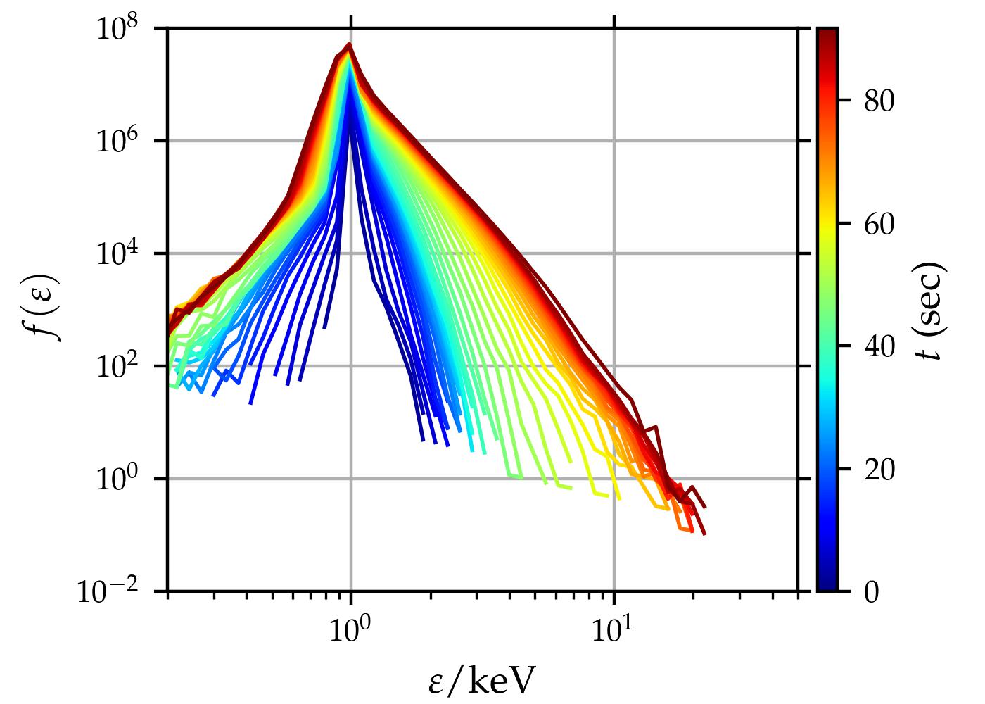
We can also get the spatial distributions of local particle distributions at the final time step. The four left panels show the electron distributions in four energy bands with corresponding scaling factors. The rightmost panel shows the vertical through the center of the reconnection region at $x=0$.

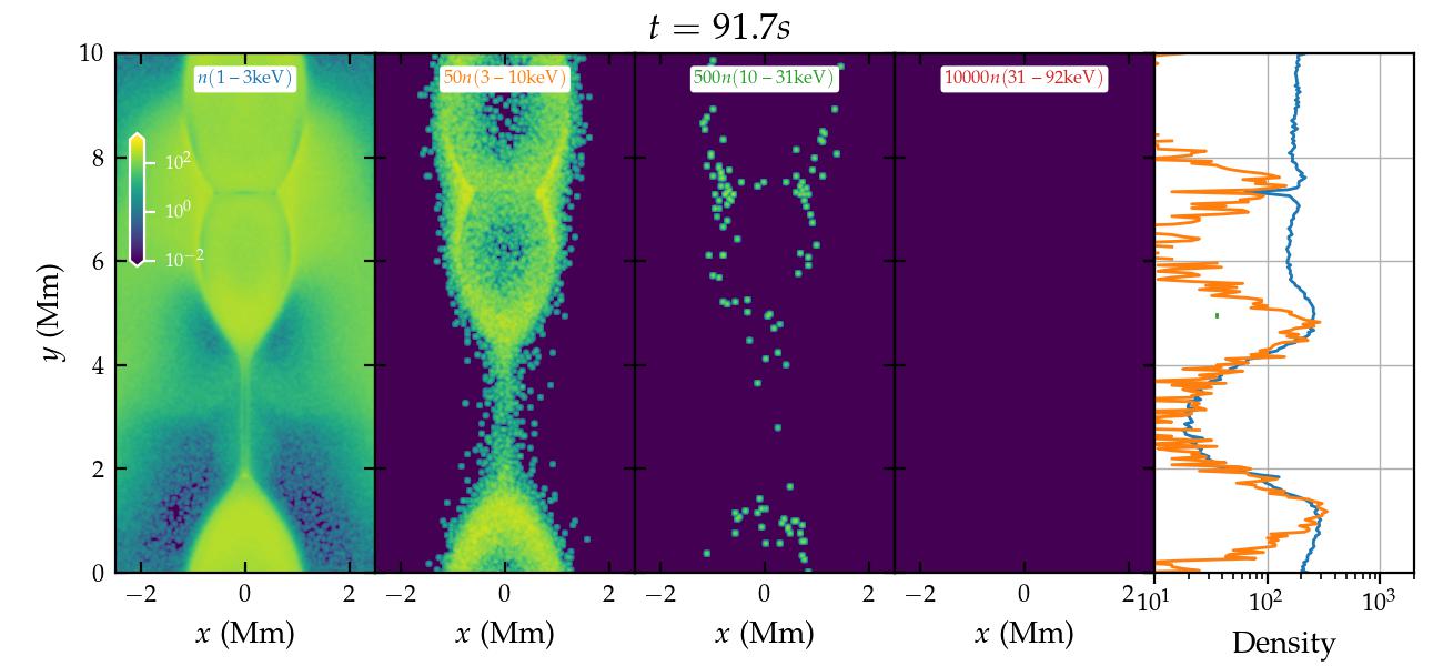
Both the spectra and the spatial distributions show that the acceleration is weak. The reason is that the compression in the MHD simulation is not strong. The acceleration will be stronger in MHD simulations with higher Lundquist numbers and resolutions.

Note

The notebook includes the script to read the global and local particle distributions. You can perform further analysis of the particle distributions.

What are not included in this description?

The code currently supports many functionalities that are not included here. Those will be gradually included in future updates of the documentation, for example,

Different particle injection methods (e.g., spatially dependent injection)
Particle-splitting techniques
Particle tracking
Momentum diffusion
Spatially dependent turbulence properties
3D simulations
Spherical coordinates